

In this part of this series, we will create a proof that our assignment satisfies the circuit we constructed in Part 1. We will convert our circuit and our assignment into polynomials and commit to them using Kate commitments and the structured reference string we created in Part 1. This will give us a list of elliptic curve points (along with a few field elements) that will serve as our proof.
To follow along with this part, you will need the parameters we set up from Part 1. In this part, we will cover matrix arithmetic, polynomial interpolation, roots of unity, cosets, and we will do some massive polynomial arithmetic. Our elliptic curve group from Part 1 has order 17. Since our proof will consist of elliptic curve points, the field we will be working over as we construct the proof is $\mathbb{F}_{17}$. All of the arithmetic in this section will be done in $\mathbb{F}_{17}$.
Some of the arithmetic we'll do is very tedious, so you may want to use some help from a calculator like WolframAlpha.
Polynomial Interpolation
Many zero-knowledge proving systems exploit a fact about polynomials that allow proofs to be succinct: if two polynomials $P$ and $Q$ are evaluated at some random input $a$, and their values happen to be the same at $a$, then the two polynomials are almost certainly identical. This is formalized in the Schwartz-Zippel lemma, commonly used in zero-knowledge proof systems.
In order to use this tool we'll have to convert the vectors that define our circuit and assignment from Part 1 into polynomials.
Two points define a line (a degree-1 polynomial), meaning for any two points there is a single line that passes through them. Similarly, three points define a parabola (a degree-2 polynomial). In general, $n$ points define a degree $n-1$ polynomial that passes through those points.
Suppose we have a vector like $\mathbf{v} = (5, 8, 13)$. We can convert the vector into a list of points ${(0,5), (1, 8), (2, 13)}$ simply using the index of the value in the vector as the $x$-coordinate. Then there is a unique degree-2 polynomial $f_\mathbf{v}$ that passes through these points. (In this case, $f_\mathbf{v}(x) = 5 + 2x + x^2$.) The process of finding this polynomial is called polynomial interpolation.
Roots of Unity
Above, we used ${0,1,2}$ as the domain for our target polynomial, but any domain can be used. In PLONK, the domain that is used for polynomial interpolation consists of roots of unity. The $n$th roots of unity of a field are the field elements $x$ that satisfy $x^n = 1$.
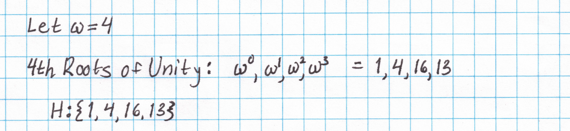
The vectors for our circuit and assignment are all of length four, so the domain of our polynomials must have at least four elements. Thankfully, the base field $\mathbb{F}_{17}$ has exactly four 4th roots of unity. Finding the 4th roots of unity in $\mathbb{F}_{17}$ isn't too difficult:
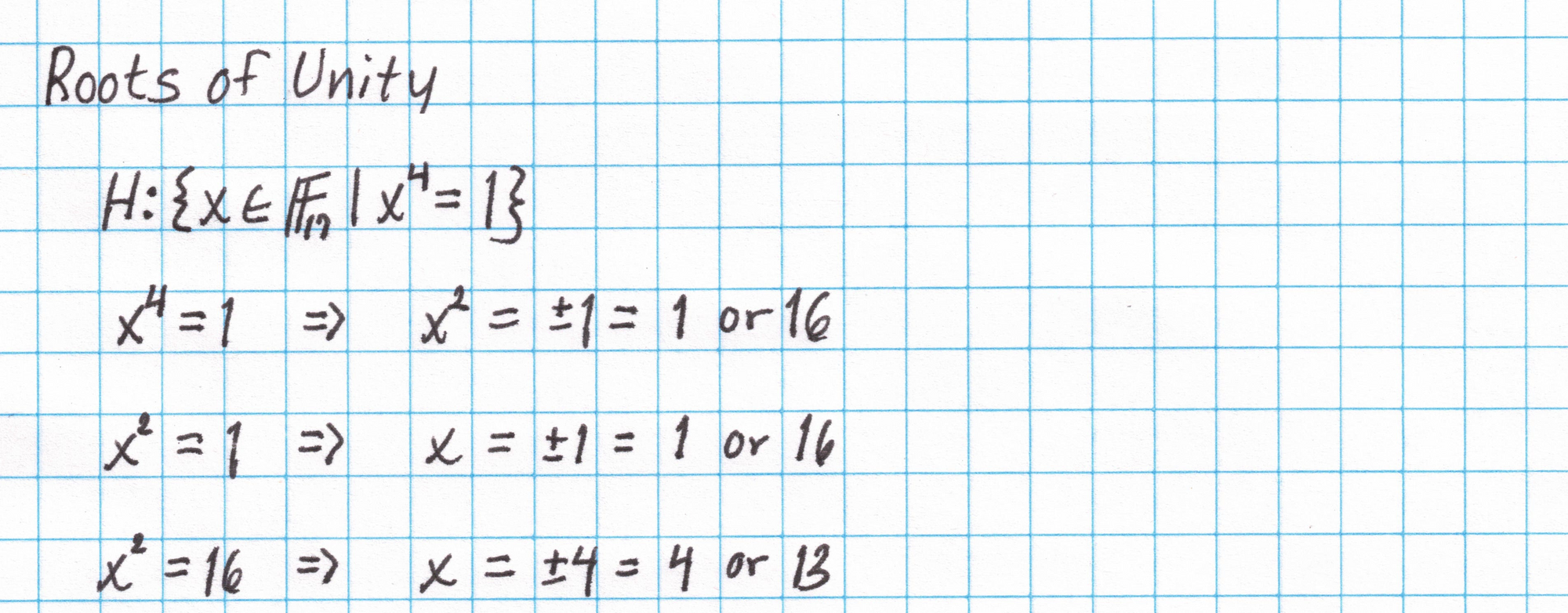
This is a multiplicative subgroup of $\mathbb{F}_{17}$ and is cyclic. We'll choose a generator $\omega$ and list the roots in order from $\omega^0$ to $\omega^3$.
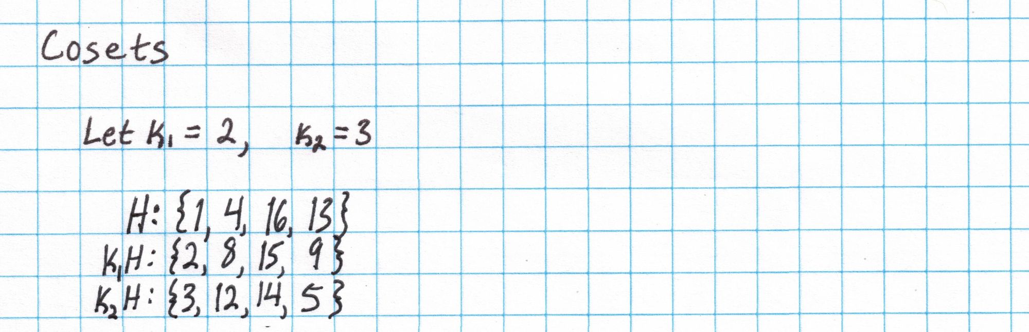
Later, we will need to label all 12 of the values in our assignment with different field elements. To do this, will use the 4 roots of unity $H$ along with two cosets of $H$. We can get these cosets by multiplying each element of $H$ by each of two constants: $k_1$ and $k_2$. The constant $k_1$ is chosen so that it is not an element of $H$, and $k_2$ is chosen so that it is neither an element of $H$ nor $k_1H$. This ensures we have 12 total field elements to use as labels.
Interpolating Using the Roots of Unity
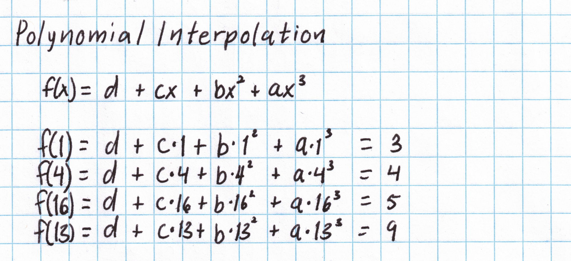
Now that we have a suitable domain $H = {1, 4, 16, 13}$ we can begin interpolating the polynomials defining our circuit. Interpolation can be done by solving a system of equations which can then be modeled with matrix arithmetic.
We will start with the first vector in our assignment $\mathbf{a} = (3,4,5,9)$. (If you are using your own assignment to the Pythagorean circuit feel free to use the computations below as a guide.) The interpolated polynomial will be degree-3 and have the form $f_{\mathbf{a}}(x) = d + cx + bx^2 + ax^3$. We want $f_{\mathbf{a}}(1) = 3$, $f_{\mathbf{a}}(4) = 4$, $f_{\mathbf{a}}(16) = 5$, and $f_{\mathbf{a}}(13) = 9$, which gives us a system of equations.
The system of equations can be rewritten as a matrix equation and solved by computing an inverse matrix.
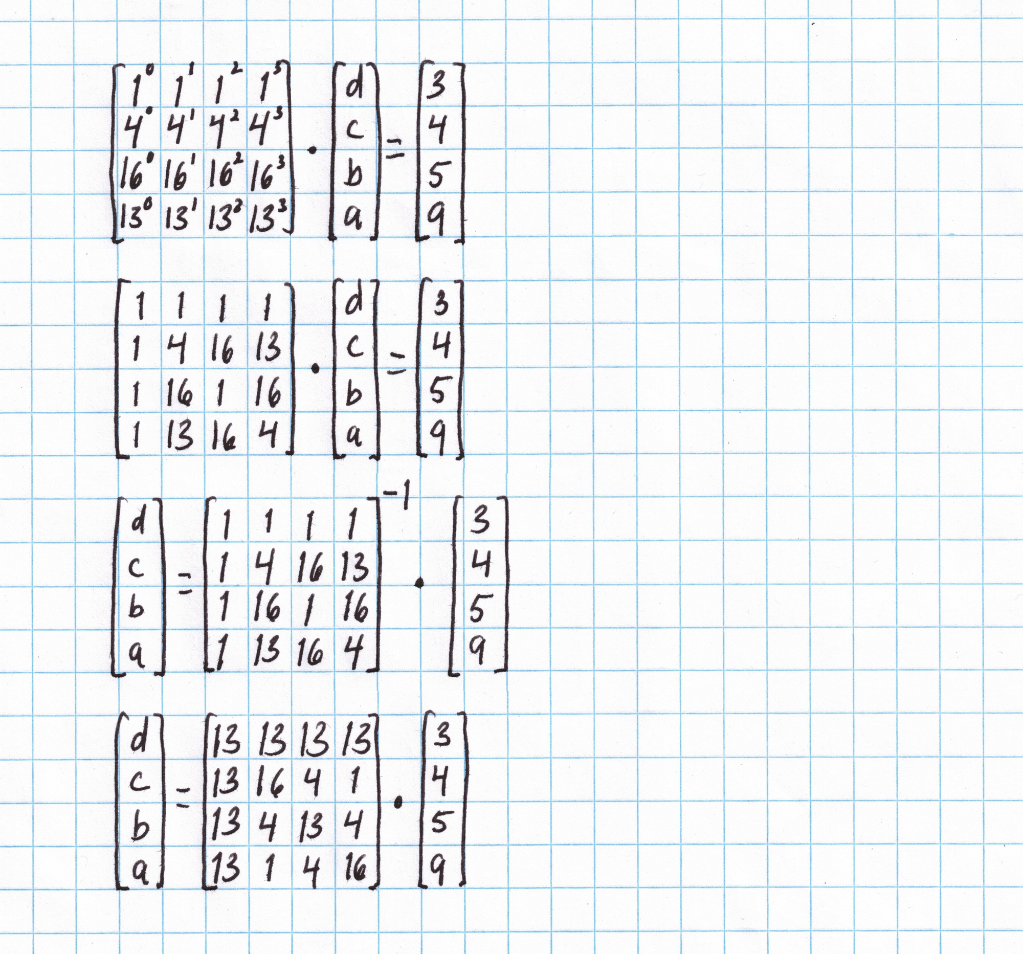
The matrix from the last step above does all the work of interpolation for us, and will work for any vector of length 4 over the domain $H$.
Now we can find the polynomial $f_{\mathbf{a}}$ by multiplying the vector $\mathbf{a} = (3,4,5,9)$ by the interpolation matrix.
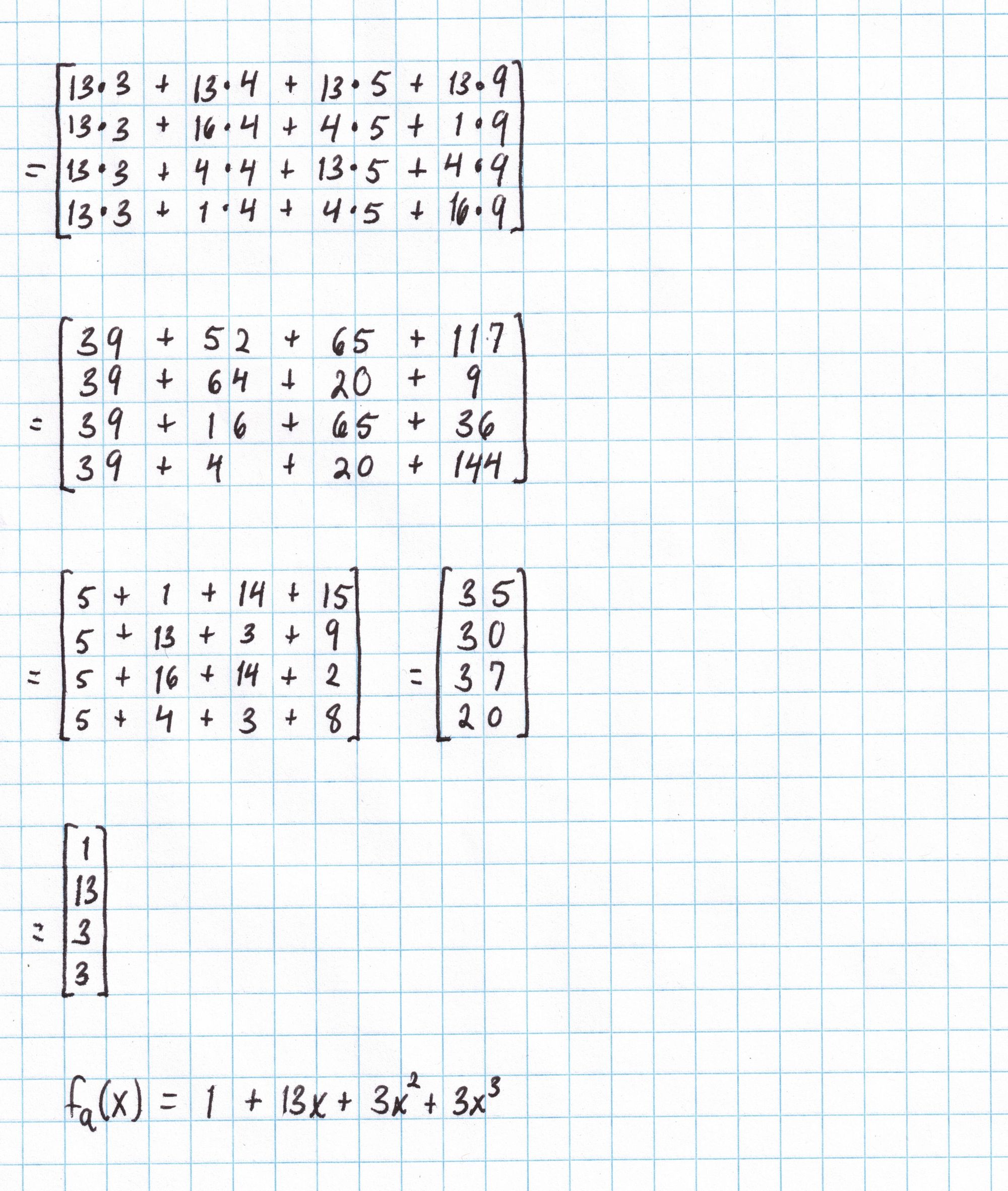
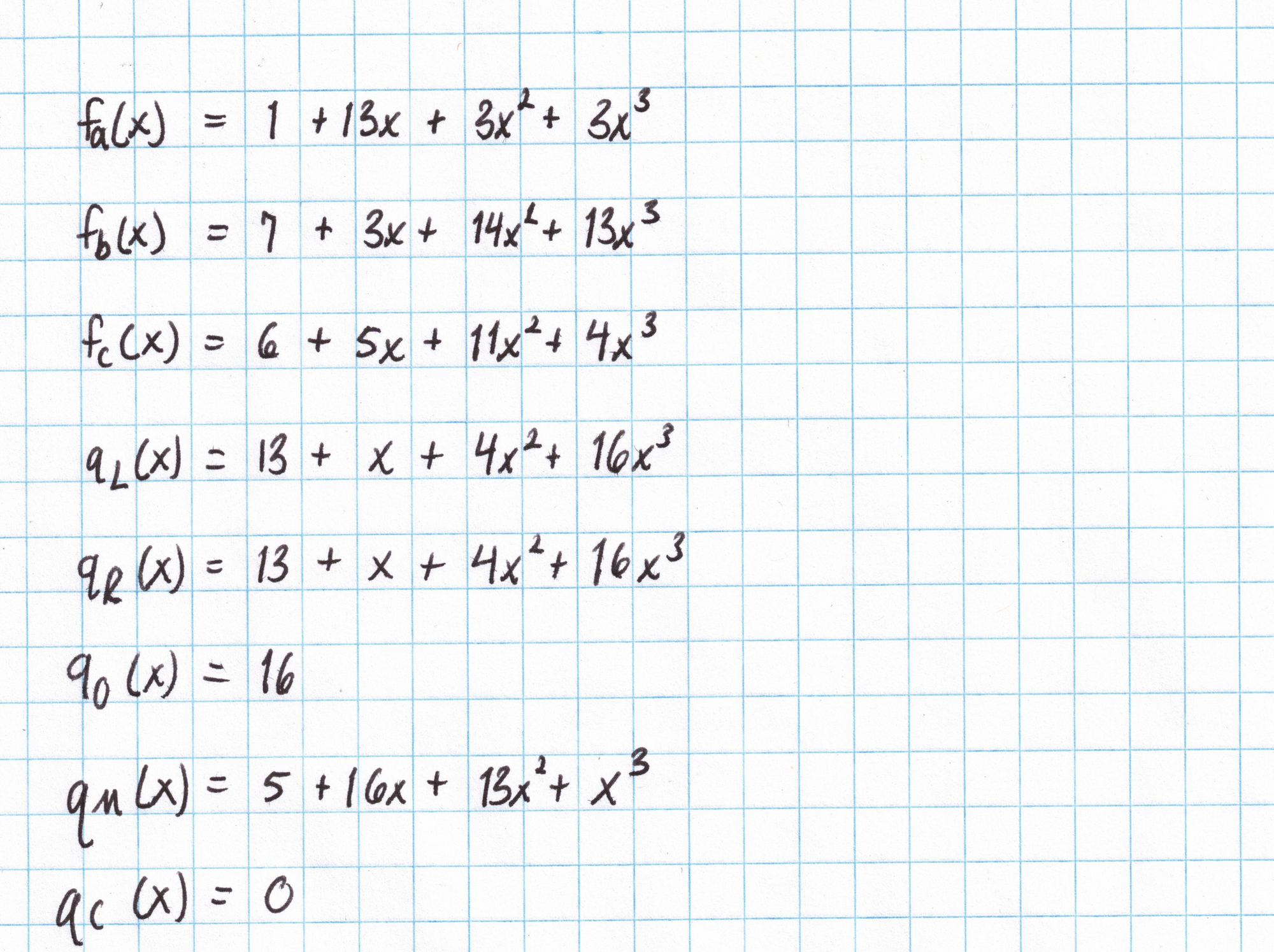
We'll need to repeat this work for all of the vectors we found in Part 1: ($\mathbf{a}$, $\mathbf{b}$, $\mathbf{c}$, $\mathbf{q_L}$, $\mathbf{q_R}$, $\mathbf{q_O}$, $\mathbf{q_M}$, and $\mathbf{q_C}$). Here are the results:
Copy Constraints
The circuit we created in Part 1 isn't quite enough to completely rule out incorrect assignments. This is because our gates are essentially disconnected from each other. The output of the first gate (9 in this example) is supposed to be the left input of the final gate, but nothing in our four gate circuit enforces this. This is where copy constraints come in. Copy constraints connect the variables between gates by forcing them to be equal.
The copy constraints involving left, right and output values are encoded as polynomials $S_{\sigma_1}$, $S_{\sigma_2}$, and $S_{\sigma_3}$ using the cosets we found earlier. The roots of unity $H$ are used to label the entries in $\mathbf{a}$, the elements of $k_1H$ are used to label the entries in $\mathbf{b}$, and $\mathbf{c}$ is labeled by the elements of $k_2H$.
Here are the copy constraints that complete our Pythagorean circuit:
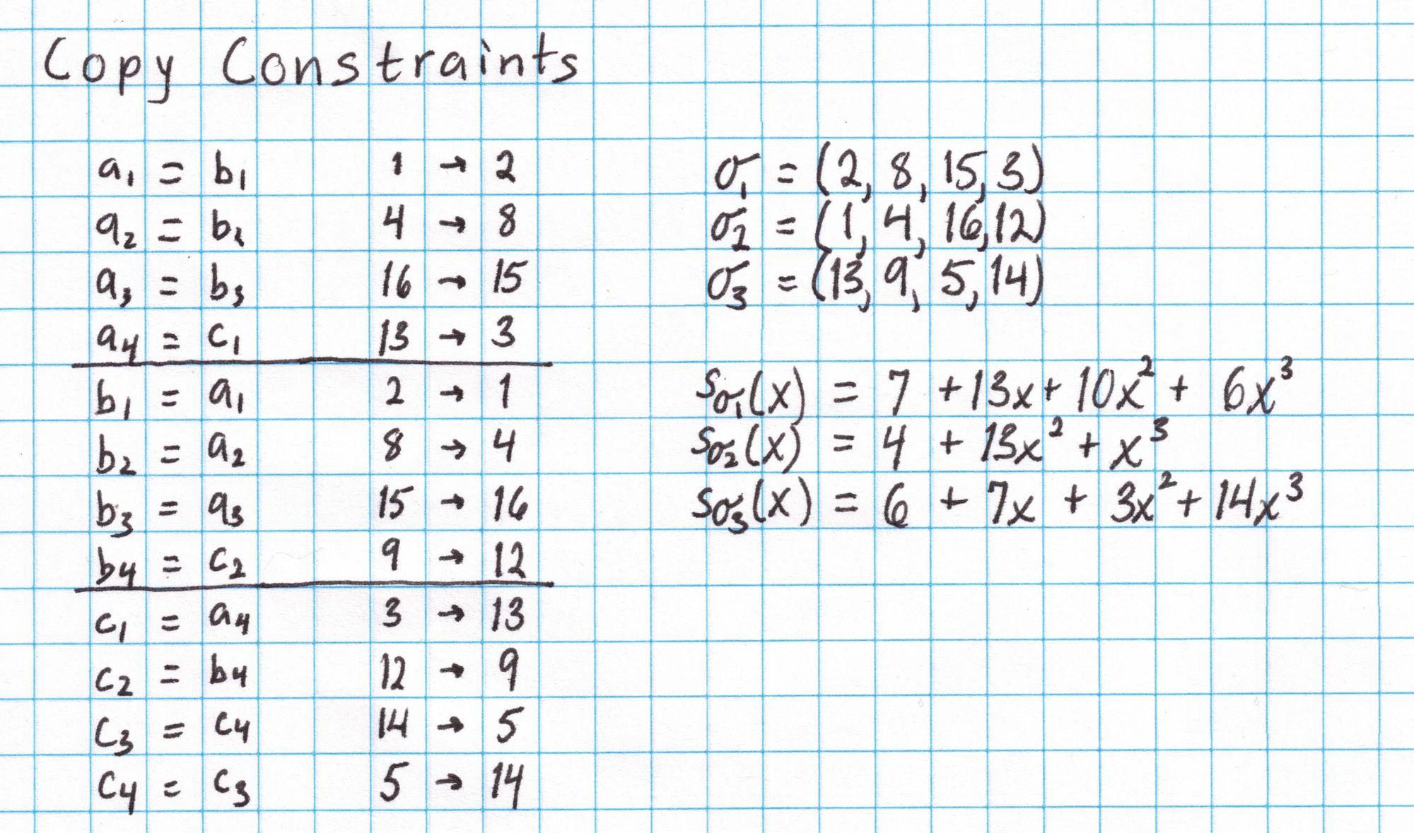
The constraint equations in the leftmost column can be thought of as a mapping between labels from our cosets. The outputs of the mapping are collected into three vectors $\sigma_1$, $\sigma_2$, and $\sigma_3$.
Now, the fact that the output of the first gate is the left input of the fourth gate is represented by the label $3$ occupying the fourth position in $\sigma_1$. The label $3$ is $k_2\cdot1$, the first element of the coset used to label outputs of each gate. Therefore, the left input of the fourth gate is the output of the first gate.
Once the vectors $\sigma_1$, $\sigma_2$, $\sigma_3$ are found, they are interpolated into the polynomials $S_{\sigma_1}$, $S_{\sigma_2}$, and $S_{\sigma_3}$.
With these interpolated polynomials we are ready to construct the proof, which occurs over five rounds.
Round 1
With the preceding calculations complete, we can move on to the first round of the Prover protocol. During each round of the protocol, we create some polynomials out of the ingredients we've already computed and typically evaluate the polynomials at some point.
Round 1 of the protocol tells us how to encode our assignment vectors $\mathbf{a},\mathbf{b},\mathbf{c}$ for later use.
Here is what we need for Round 1:
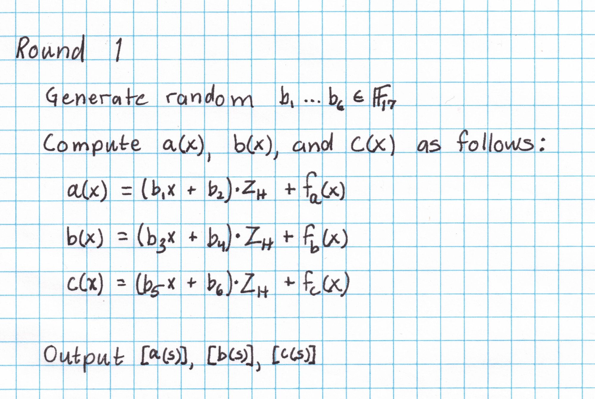
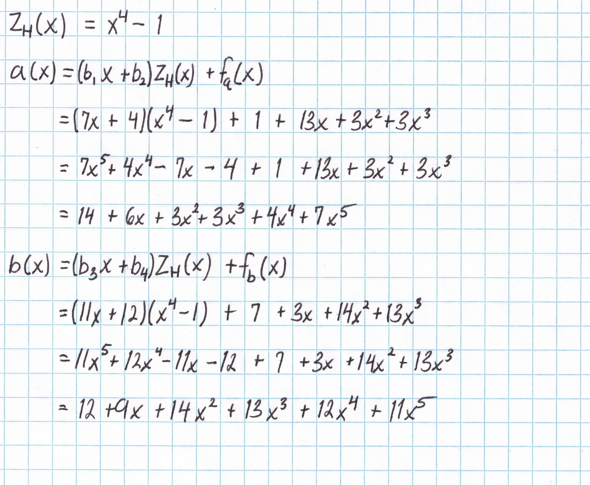
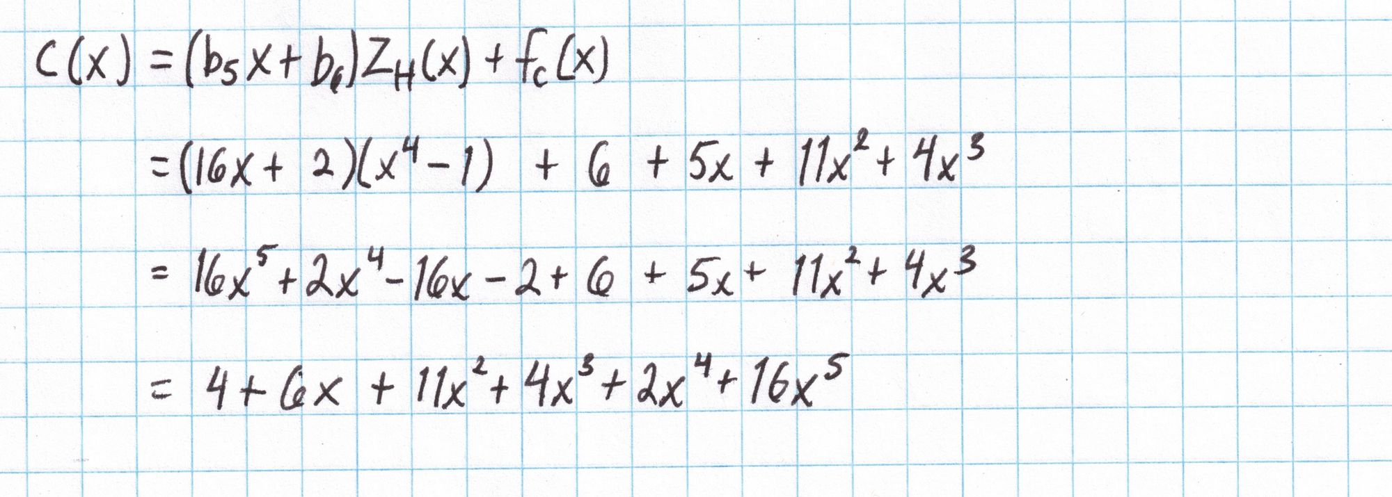
The polynomial $Z_H$ is the polynomial that is zero on all the elements of our subgroup $H$. Since $H$ is just the 4th roots of unity in our field, the polynomial $Z_H$ is easy to compute. Each 4th root of unity $x$ satisfies $x^4 = 1$, so the polynomial $x^4-1=0$ for all elements in $H$.
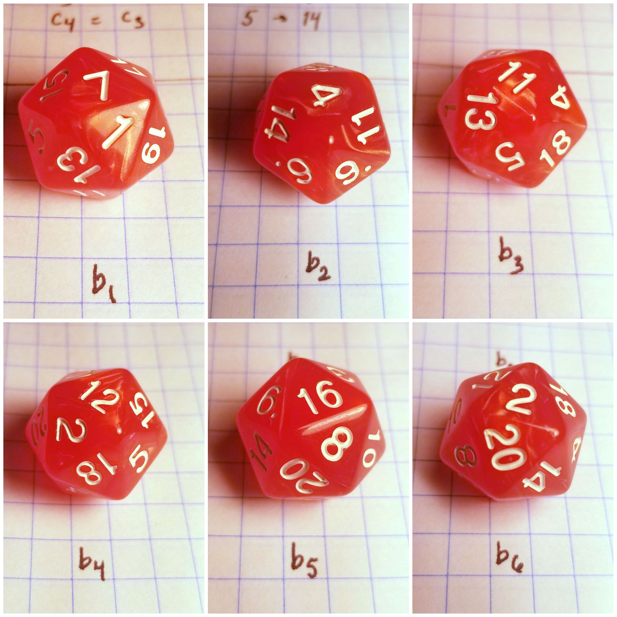
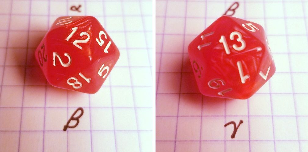
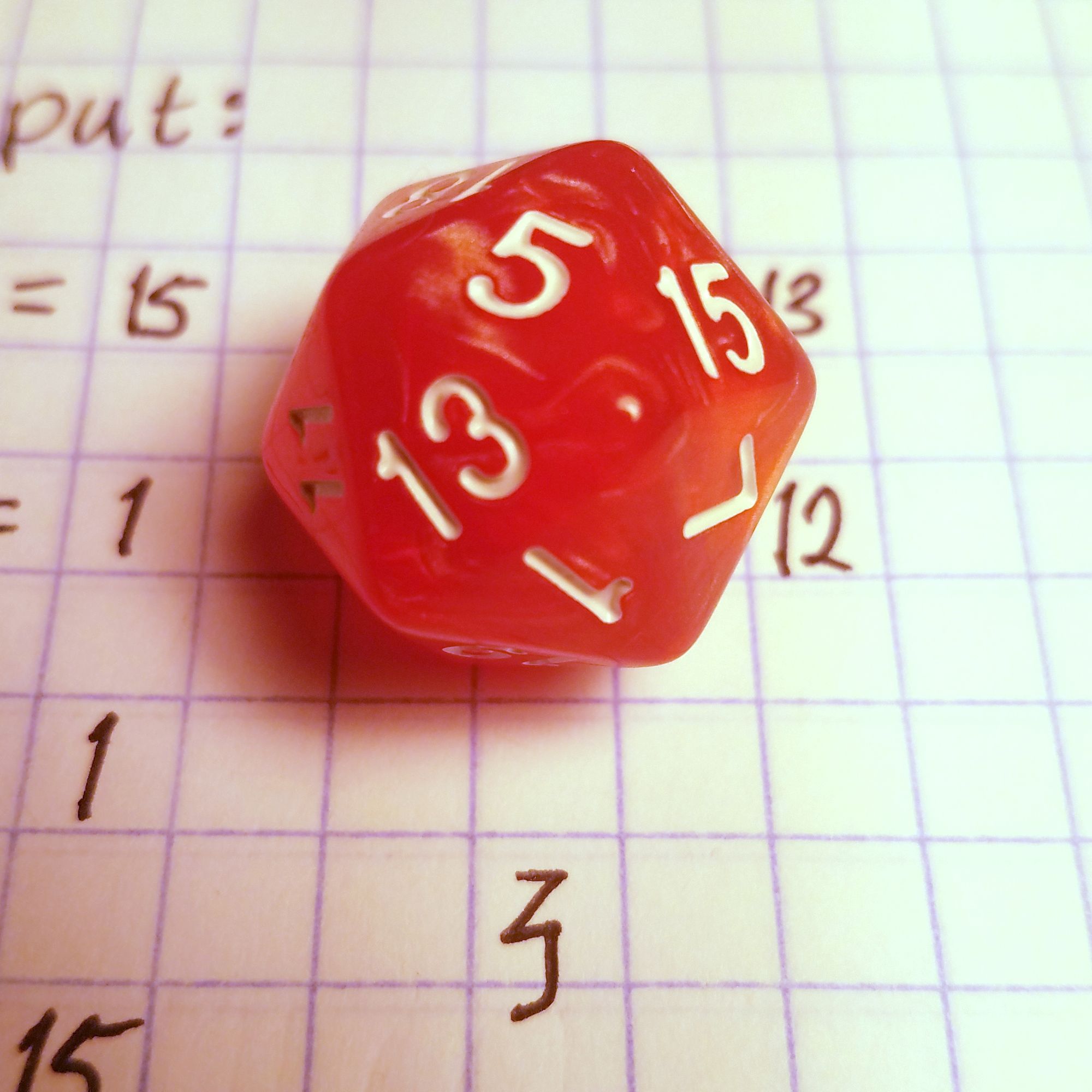
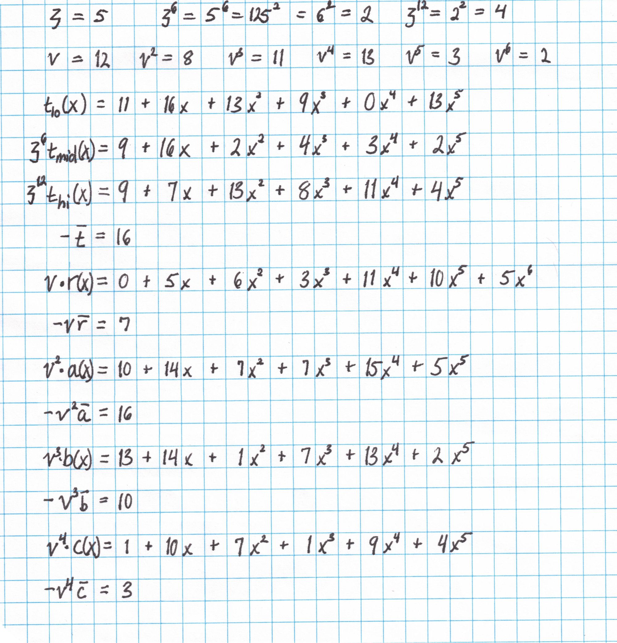
Next we'll generate six random elements of our field using a twenty-sided die. These field elements provide some hiding for our polynomials.
With these field elements and the polynomial $Z_H$, and the interpolated polynomials $f_a$, $f_b$, and $f_c$ we compute $a(x)$, $b(x)$, and $c(x)$ according to the protocol.
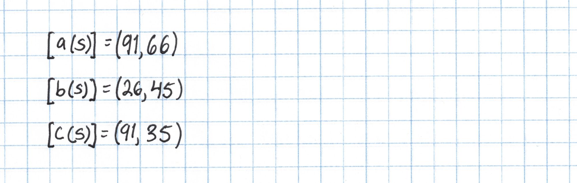
Now we compute $\left[a(s)\right]$,$\left[b(s)\right]$, and $\left[c(s)\right]$---elliptic curve points which represent these polynomials evaluated at the "secret" number $s$. We can do this using the SRS from the setup phase. A real Prover would need to use the algorithms for adding and scaling elliptic curve points from the SRS in order to compute these points. Since our elliptic curve group is small and we have a table of all the points as multiples of our generator, we can cheat using our table and save a lot of time. (How to cheat: To compute $nP + mQ$, first look up $P$ and $Q$ in the table and write them as multiples of the generator $(1,2)$. Now $nP+mQ = nk(1,2) + ml(1,2)$ for some $k$ and $l$ from the table. Then $nk(1,2) + ml(1,2) = (nk+ml)(1,2)$. Reduce $nk+ml$ mod 17 and use the table again to look up the result.)
Here is the calculation of $\left[a(s)\right]$ using the SRS from the setup phase and the "cheat" from above:
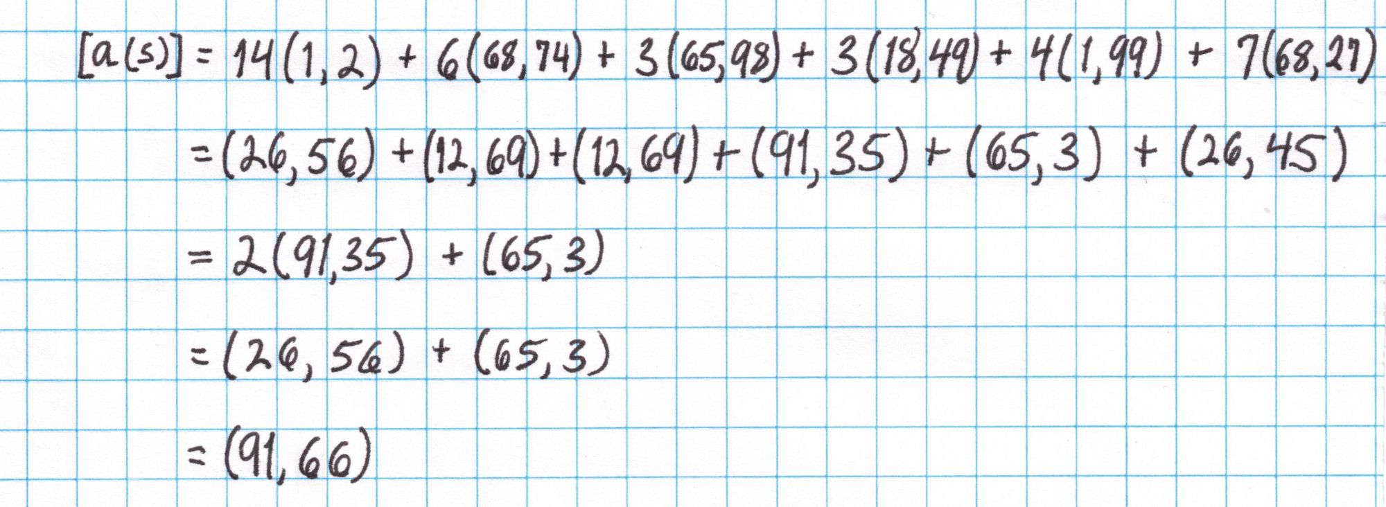
We repeat this for $\left[b(s)\right]$ and $\left[c(s)\right]$ and output all three points. These points are commitments to polynomials representing our chosen assignments to the Pythagorean circuit.
Round 2
Round 2 is about committing to a single polynomial $z$ that encodes all of the copy constraints we discussed earlier.
Here is what we need for Round 2:
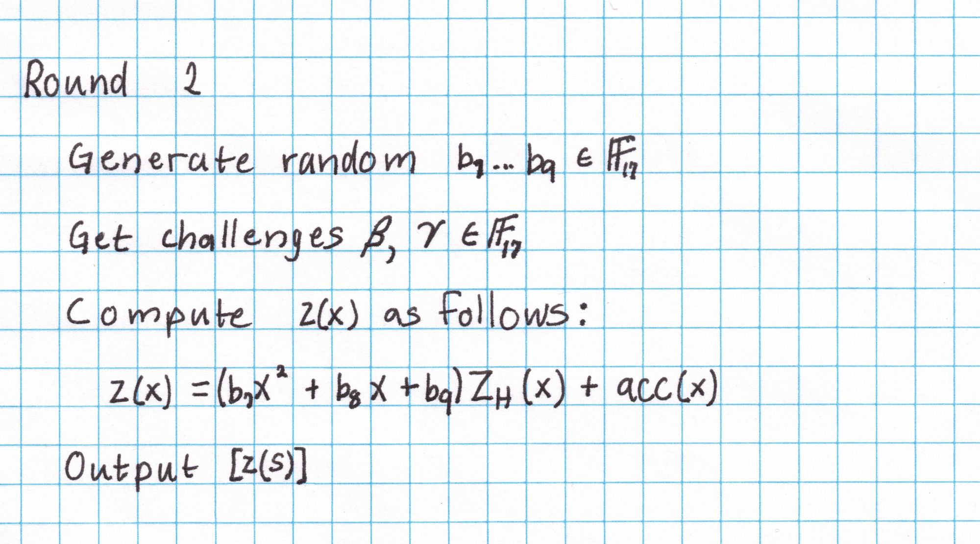
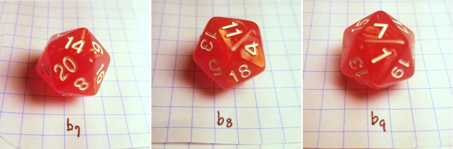
The random $b_7,b_8,b_9$ can be found with a dice roll by the Prover.
In Round 2 we see the first use of "challenge" values, in this case $\beta$ and $\gamma$. The nature of these challenge values depends on whether the protocol is interactive. In an interactive protocol, the Verifier chooses these challenge values and sends them to the Prover, who uses them to construct the proof. In a non-interactive protocol, these values are derived from a cryptographic hash of a transcript of the Prover's process. These values would be unpredictable by the either the Prover or Verifier, but each party is be able to compute the same challenge values using the same hash function on the transcript. This is known as the Fiat-Shamir transform which can turn an interactive protocol non-interactive.
For simplicity, we will imagine an interactive protocol where the Verifier sends these challenge values to the Prover.
The Verifier chooses random $\beta$ and $\gamma$ and sends them to the Prover.
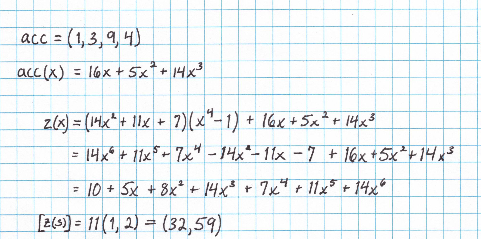
The polynomial $z$ is constructed from an accumulator vector that is defined like this:

Notice each accumulator value is multiplied by the one before it. Also, because of the way we defined the $S_\sigma$ polynomials earlier, many of the factors in the numerator and denominator will cancel out. For instance, since $b_2$ = $a_2$ and $S_{\sigma_1}(4) = k_14$, the factors $(b_2 +\beta k_1 \omega^1 + \gamma)$ from the numerator exactly equals $(a_2 +\beta S_{\sigma_1}(\omega^1) + \gamma)$ from the denominator and will cancel out. Typically there will be some factors remaining that do not cancel.
Here is the accumulator vector computed for our assignment and challenge values:
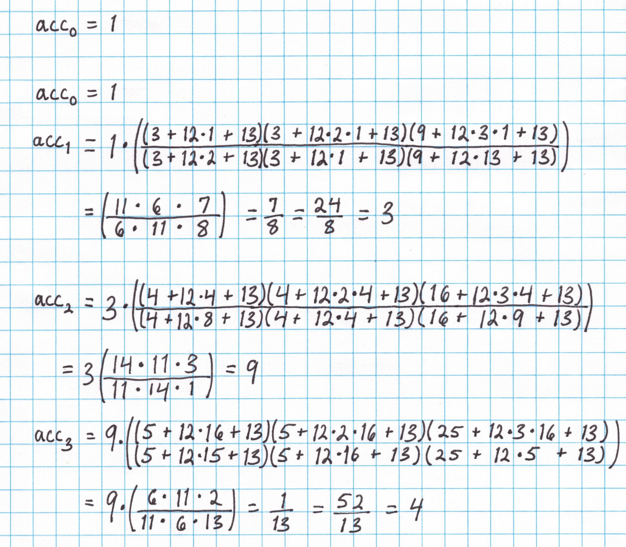
The accumulator vector is interpolated into a polynomial $acc(x)$ and this is used to create the polynomial $z$. Then $z$ is evaluated at the secret number $s$ using the SRS from the setup.
Round 3
Next comes the most massive computation of the entire protocol. Our goal is to compute the polynomial $t$, which will be of degree $3n+5$ for $n$ gates. The polynomial $t$ encodes the majority of the information contained in our circuit and assignments all at once. Here is the procedure for Round 3:
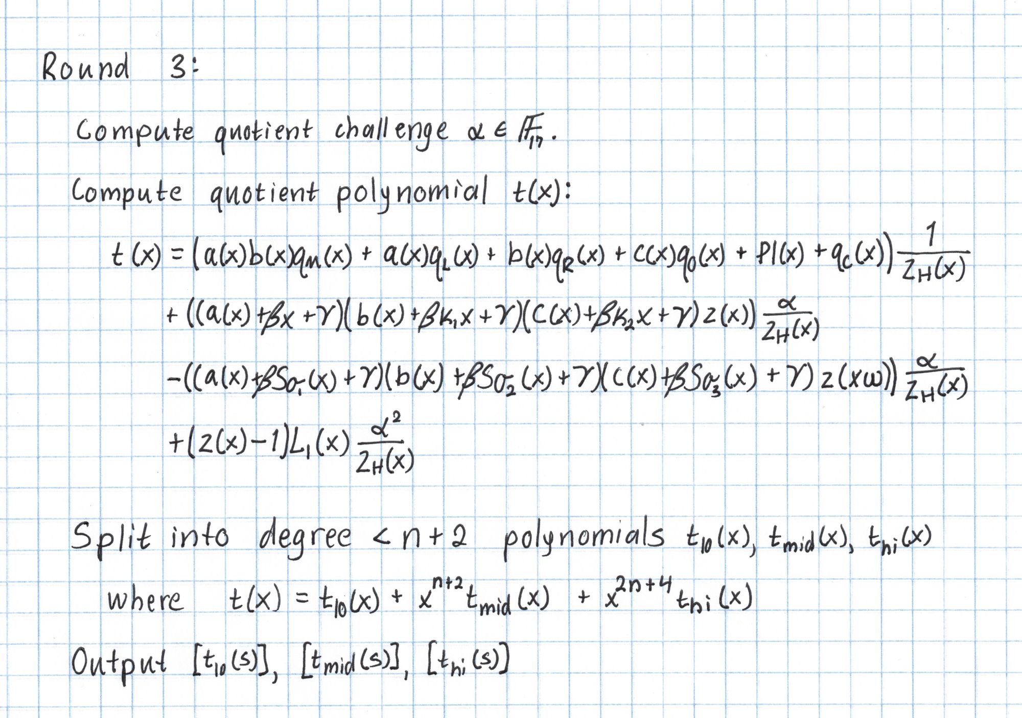
The last line of the $t$ definition has a reference to a polynomial $L_1$ which we haven't seen yet. $L_1$ refers to a Lagrange basis polynomial over our roots of unity $H$. Specifically $L_1(1) = 1$, but takes the value 0 on each of the other roots of unity. The coefficients for $L_1$ can be found by interpolating the vector $(1,0,0,0)$ to get $L_1(x) = 13+13x+13x^2+13x^3$.
Ther Verifier chooses random $\alpha$ and sends it to the Prover.
Some of the polynomial computations in Round 3 are very large, even for a small circuit like ours, and doing them all by hand is time consuming. If you are following along, you may want to use WolframAlpha or some other tool for this polynomial arithmetic. To keep in the spirit of PLONK by Hand, the first product of polynomials in $t$ is computed by hand below. The rest is done with computational help.
First find the product $a(x)b(x)$:
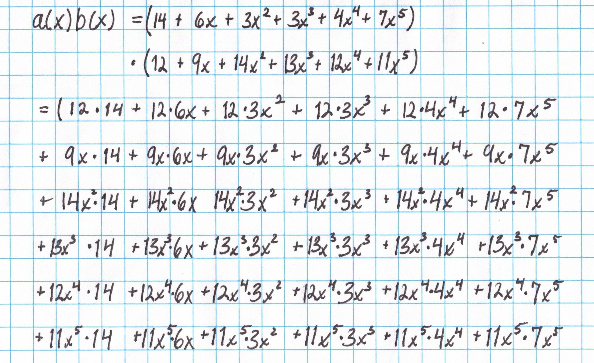
Multiplication is done term-by-term to yield monomials for each term. Terms on the diagonals that run from the lower-left to upper-right have the same degree and can be summed.
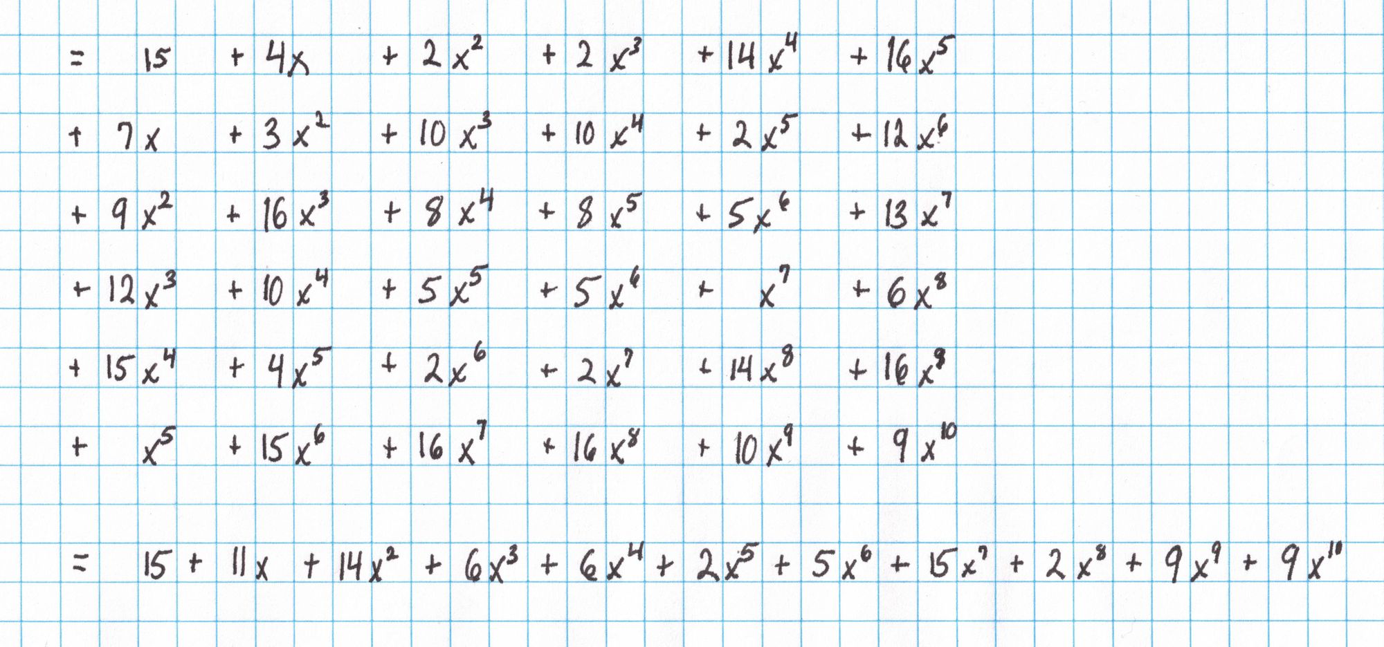
Now we can multiply $a(x)b(x)$ by $q_M(x)$ in the same fashion.
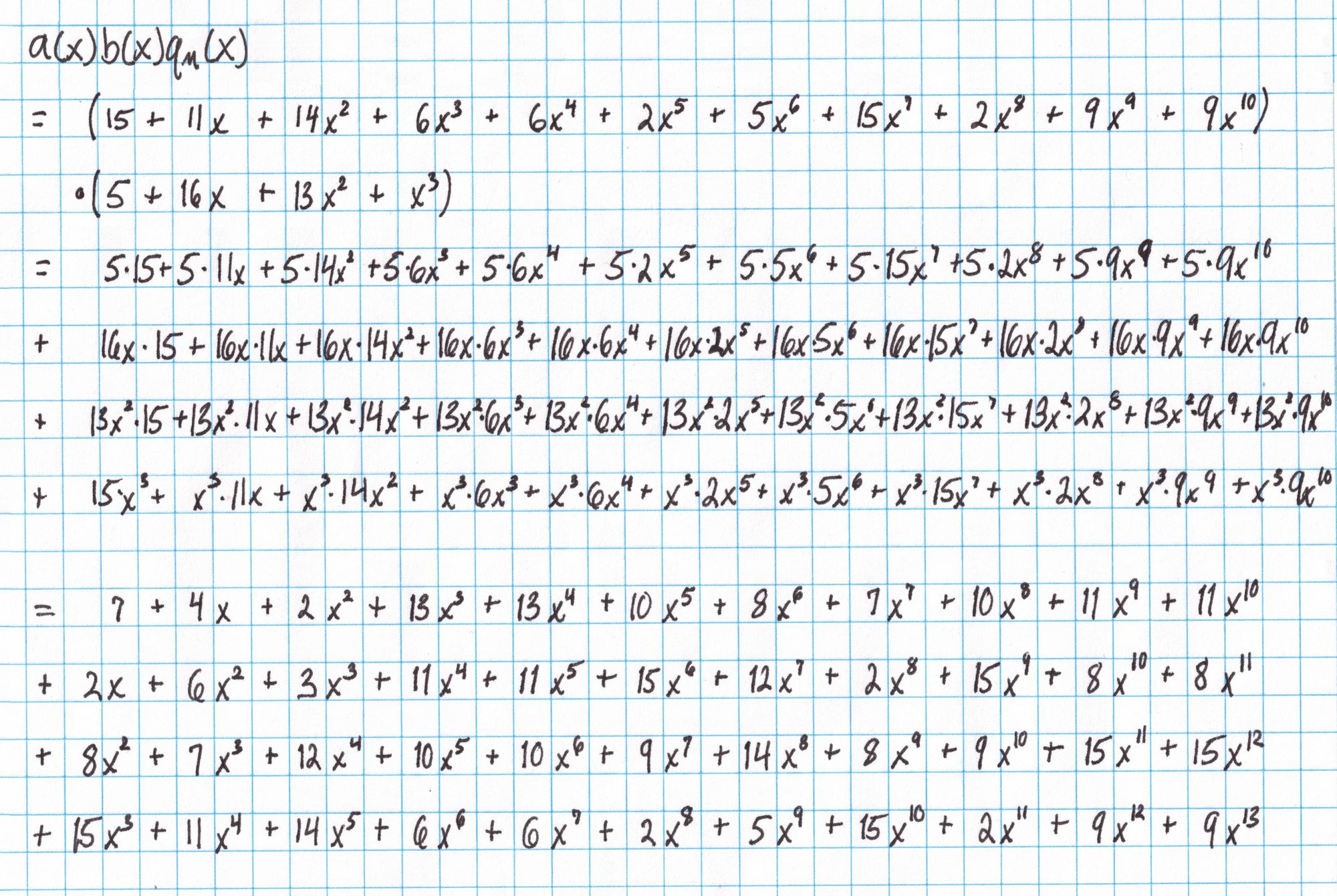
Combining along diagonals finally gives $a(x)b(x)q_M(x)$:

Now we use a calculator to get the rest of the pieces of $t$. Note that first we actually find $t(x)\cdot Z_H(x)$. We will divide out $Z_H(x)$ later in one step. To save space on the page we are representing each polynomial as a vector of its coefficients from lowest to highest degree. The four $t_i(x)Z_H(x)$ polynomials near the end of this reference correspond to the four lines of the definition of $t$ given above. You can check that these four polynomials add to the $t(x)Z_H(x)$ given on the final line.
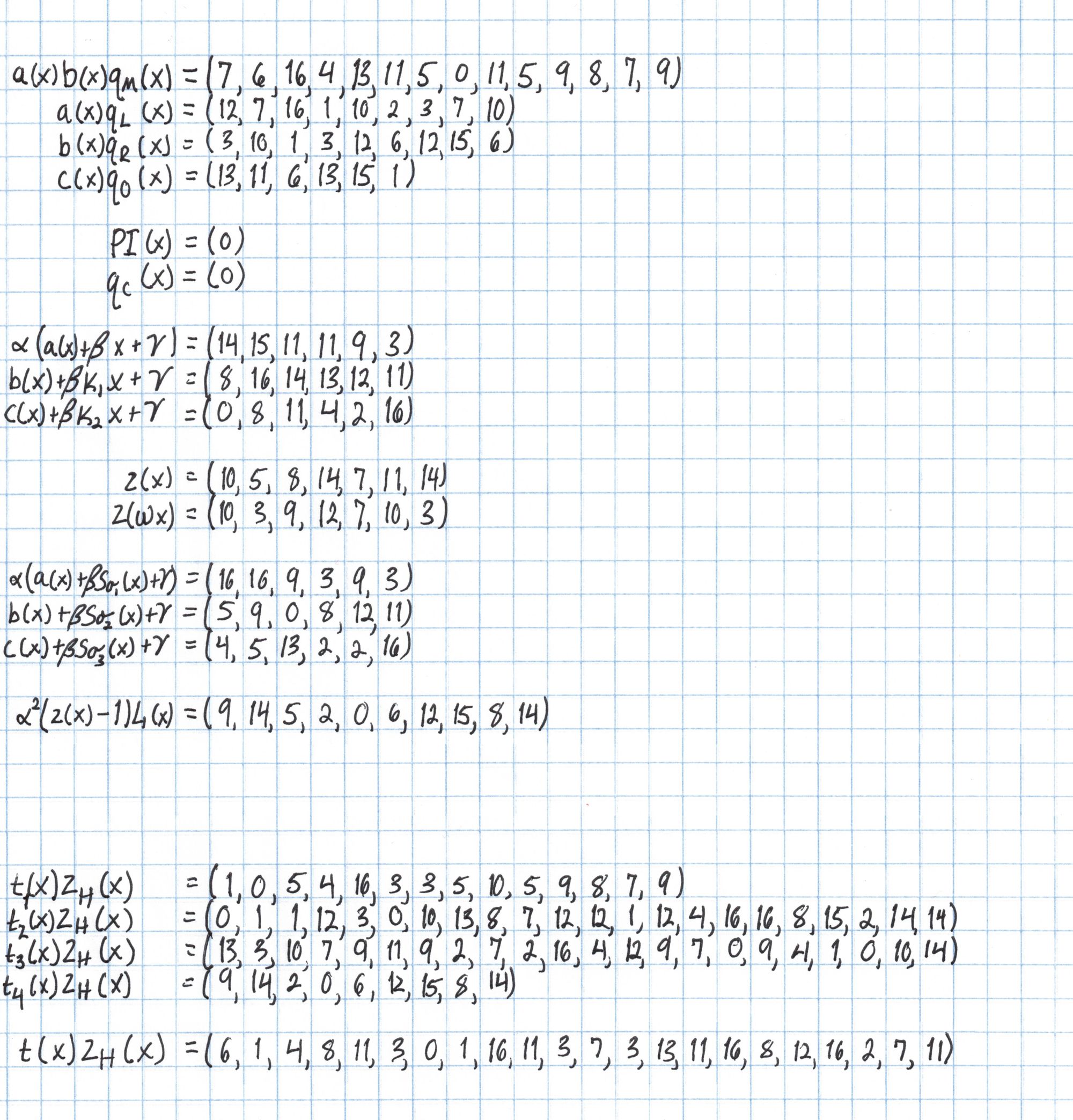
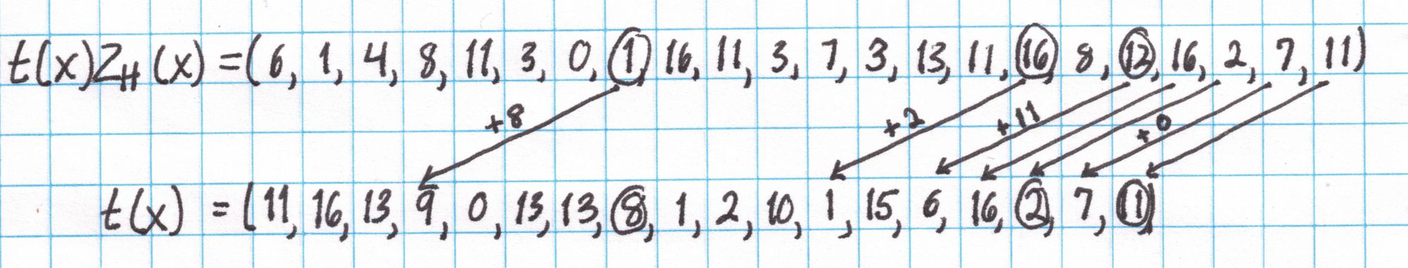
Now we divide $t(x)Z_H(x)$ by $Z_H(x) = x^4 -1$ using an algorithm similar to synthetic divsion. Since $Z_H$ is such a sparse polynomial this division is very easy. Working right to left, take each coefficient and add the coefficient directly below it from the quotient. (If there isn't a coefficient there, consider it $0$). Write this sum in the quotient underneath the coefficient 4 spaces to the left of the original. Here's a diagram showing this division:
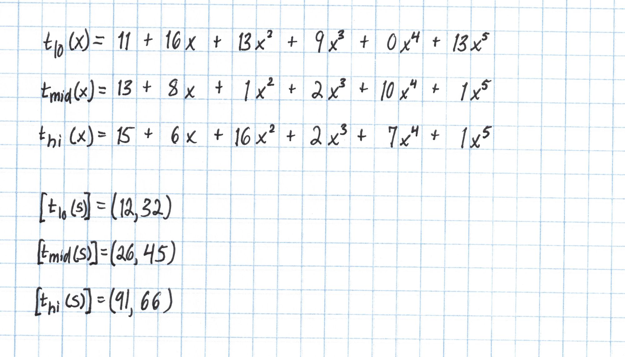
It turns out that for $n$ constraints, $t$ will have degree $3n+5$, which is too large to use the SRS from the setup phase in Part 1. However we can break $t$ into three parts of degree $n+1$ each. Each of these polynomials will use $n+2$ coefficients from $t(x)$. After dividing into three parts, we evaluate each part at $s$ using the SRS.
Round 4
In Round 4, we create a polynomial $r$ that is a kind of partner to $t$, where many of the polynomials that were included in $t$ are replaced by field elements that are evaluations of those polynomials at a challenge value $\mathfrak{z}$.
Here is what we need for Round 4:
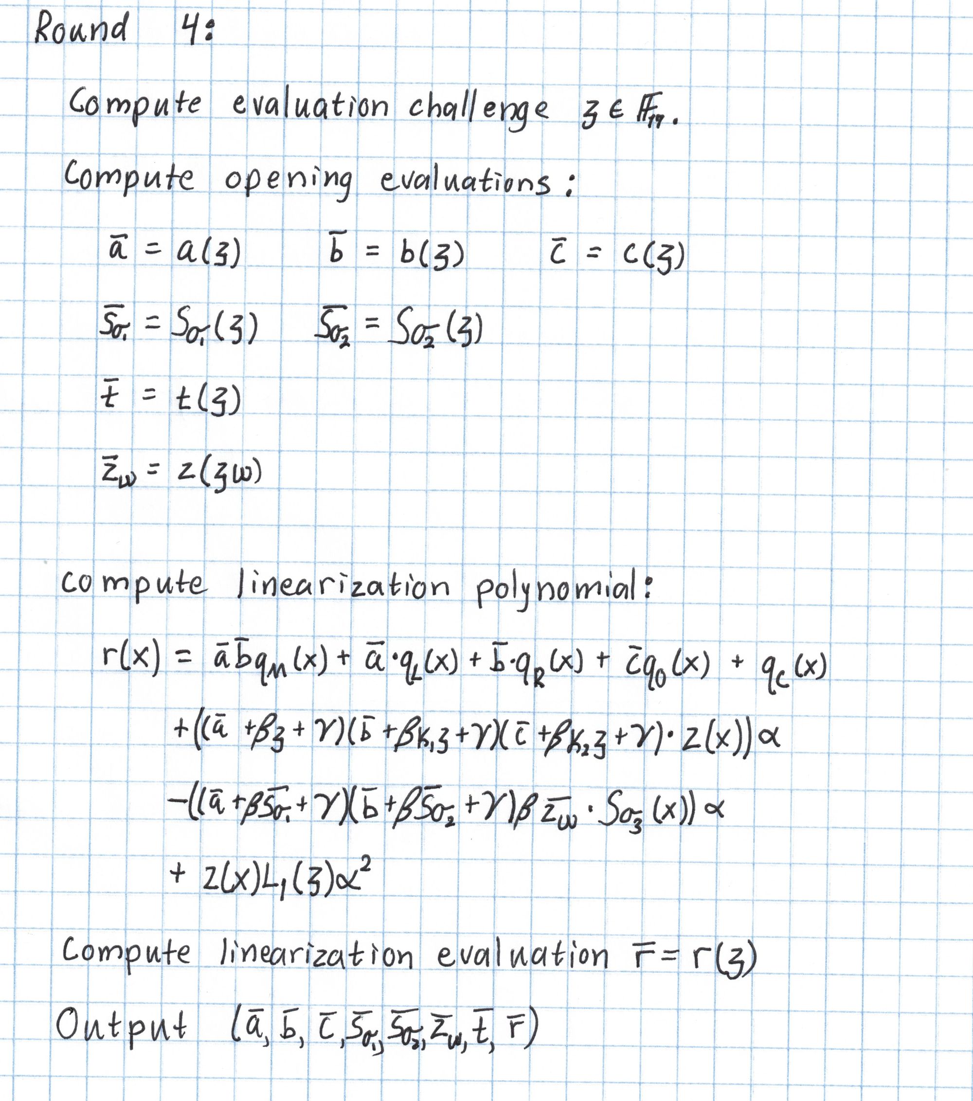
First the Verifier chooses a random $\mathfrak{z}$ and sends it to the Prover.
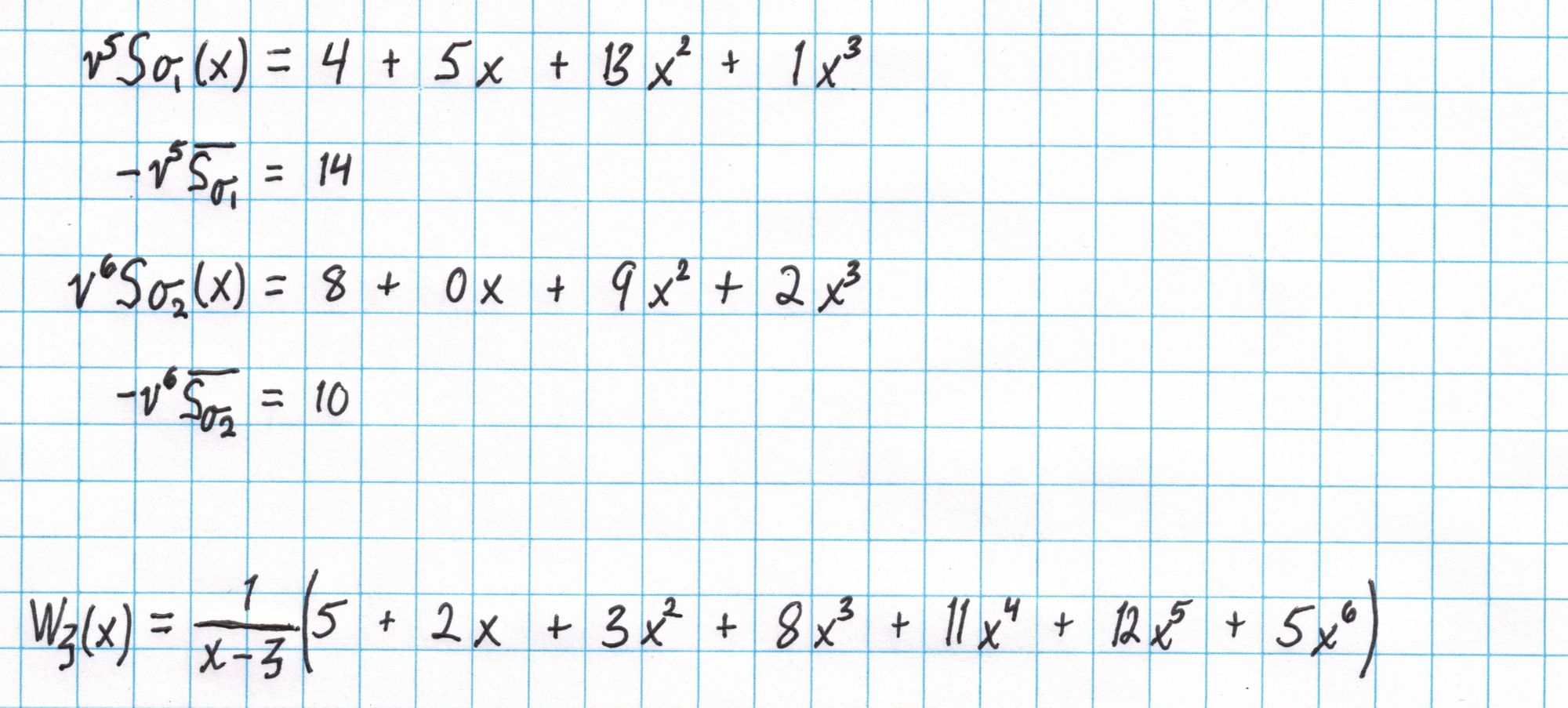
First we compute the opening evaluations of our polynomials at $\mathfrak{z}$. We show the computation for $\bar{a}=a(\mathfrak{z})$.
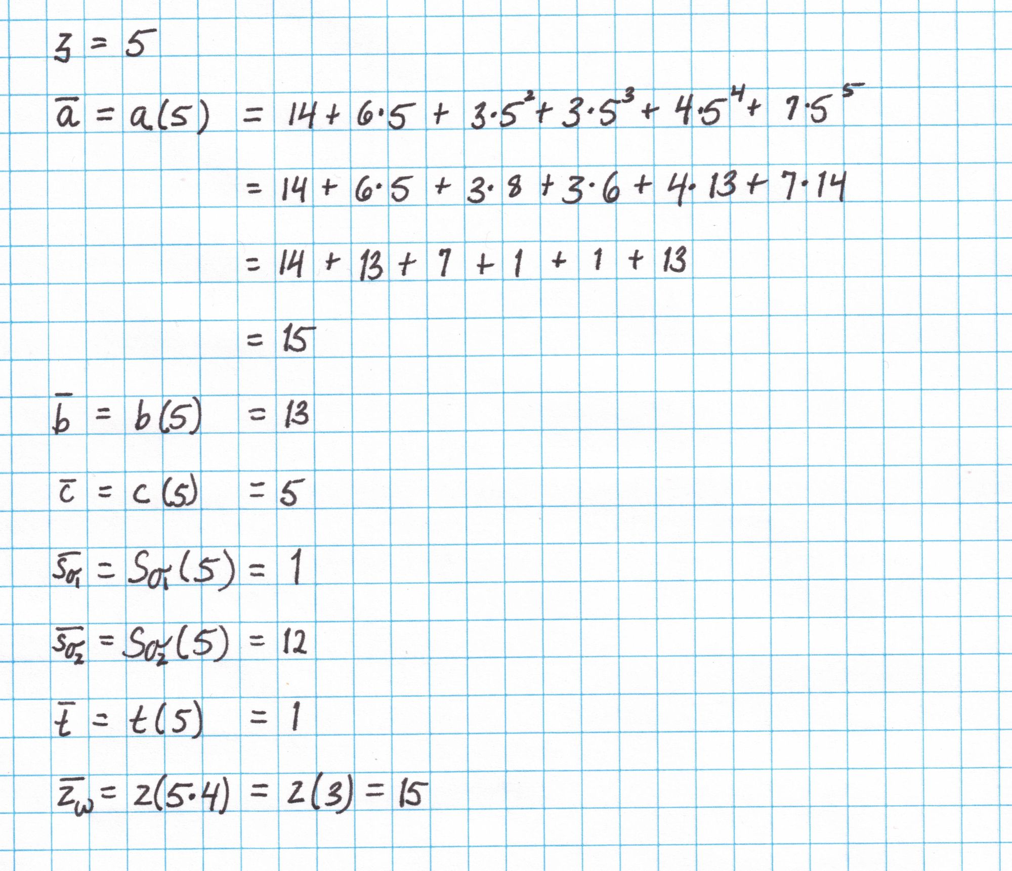
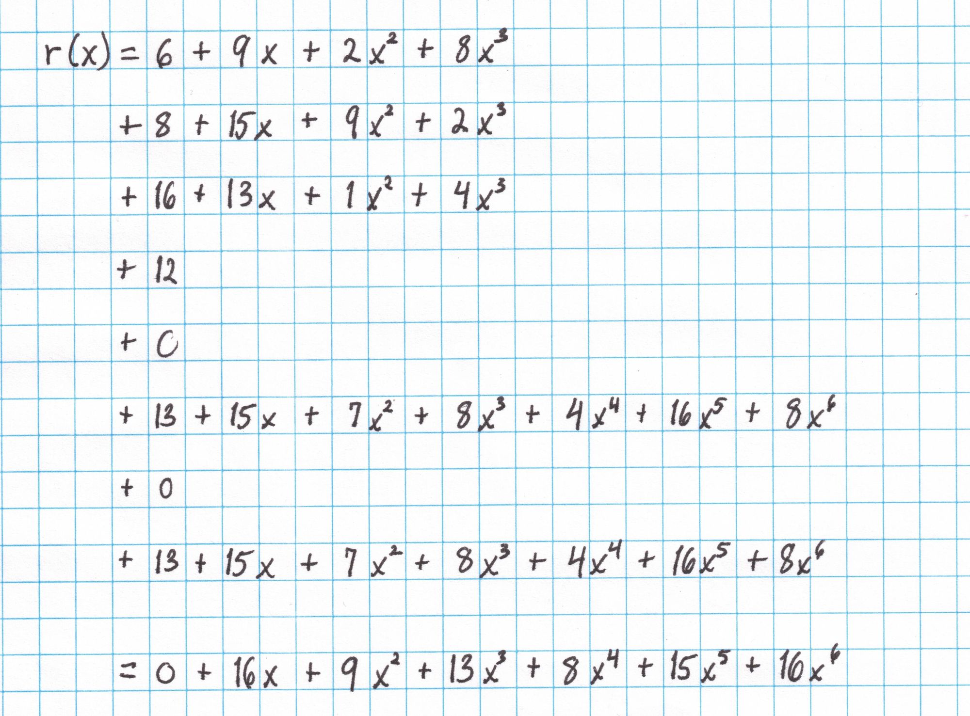
With these elements we can construct $r$ with out much trouble. Here is the full computation of $r$:
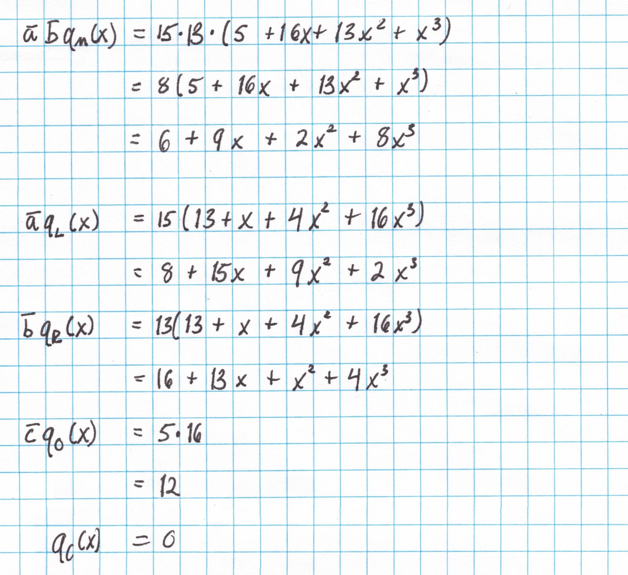
Now we add all the pieces together to get $r$.
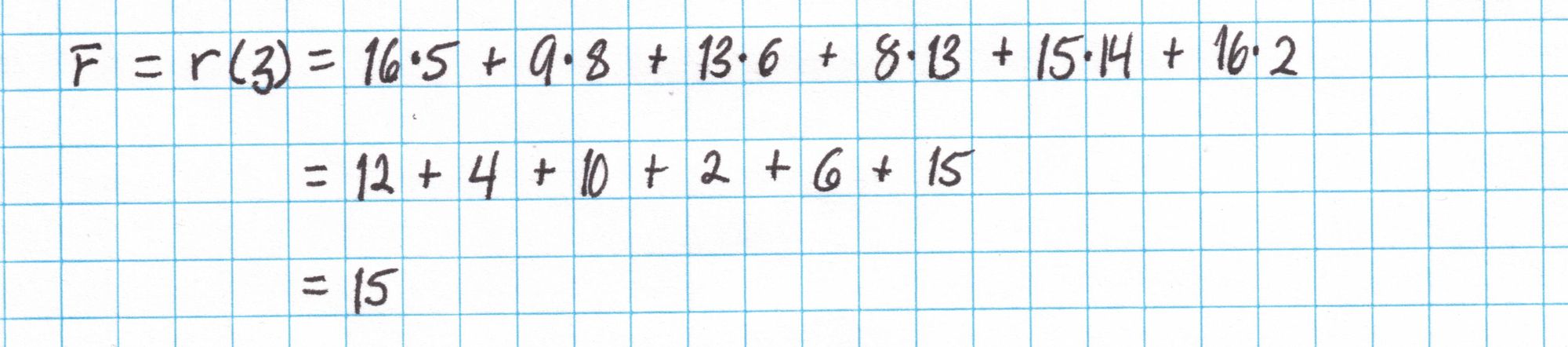
We use $r$ to compute $\bar{r}=r(\mathfrak{z})$.
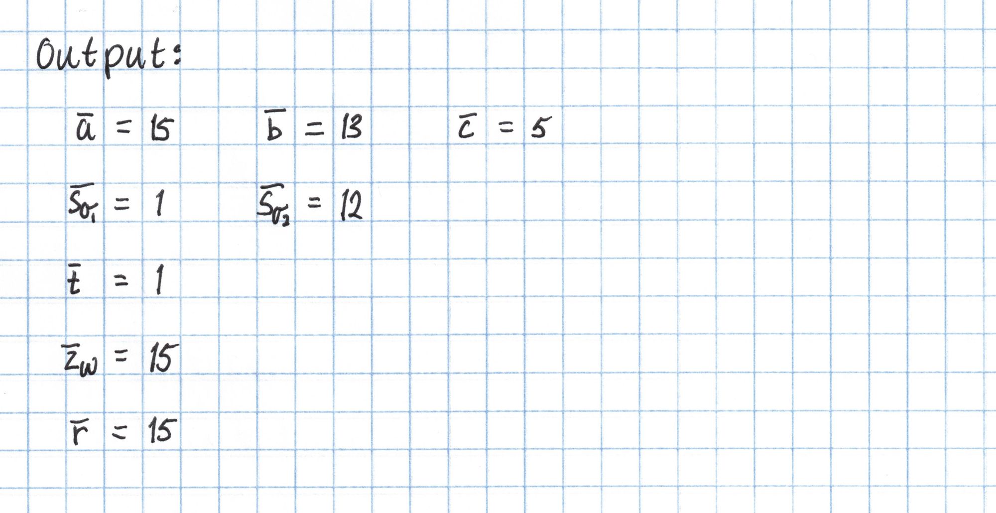
Now we output all the opening evaluations we computed in Round 4.
Round 5
We're nearly done! In Round 5, we create two large polynomials that combine all the polynomials we've been using so far and we output commitments to them.
Here is Round 5:
The Verifier chooses a random $v$ and sends it to the Prover.

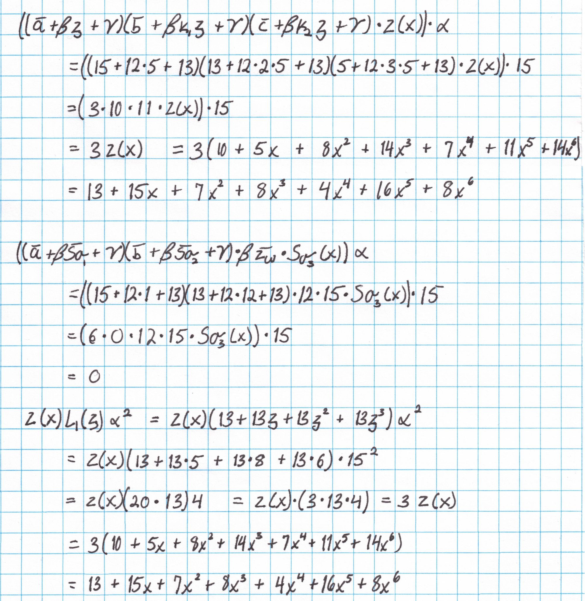
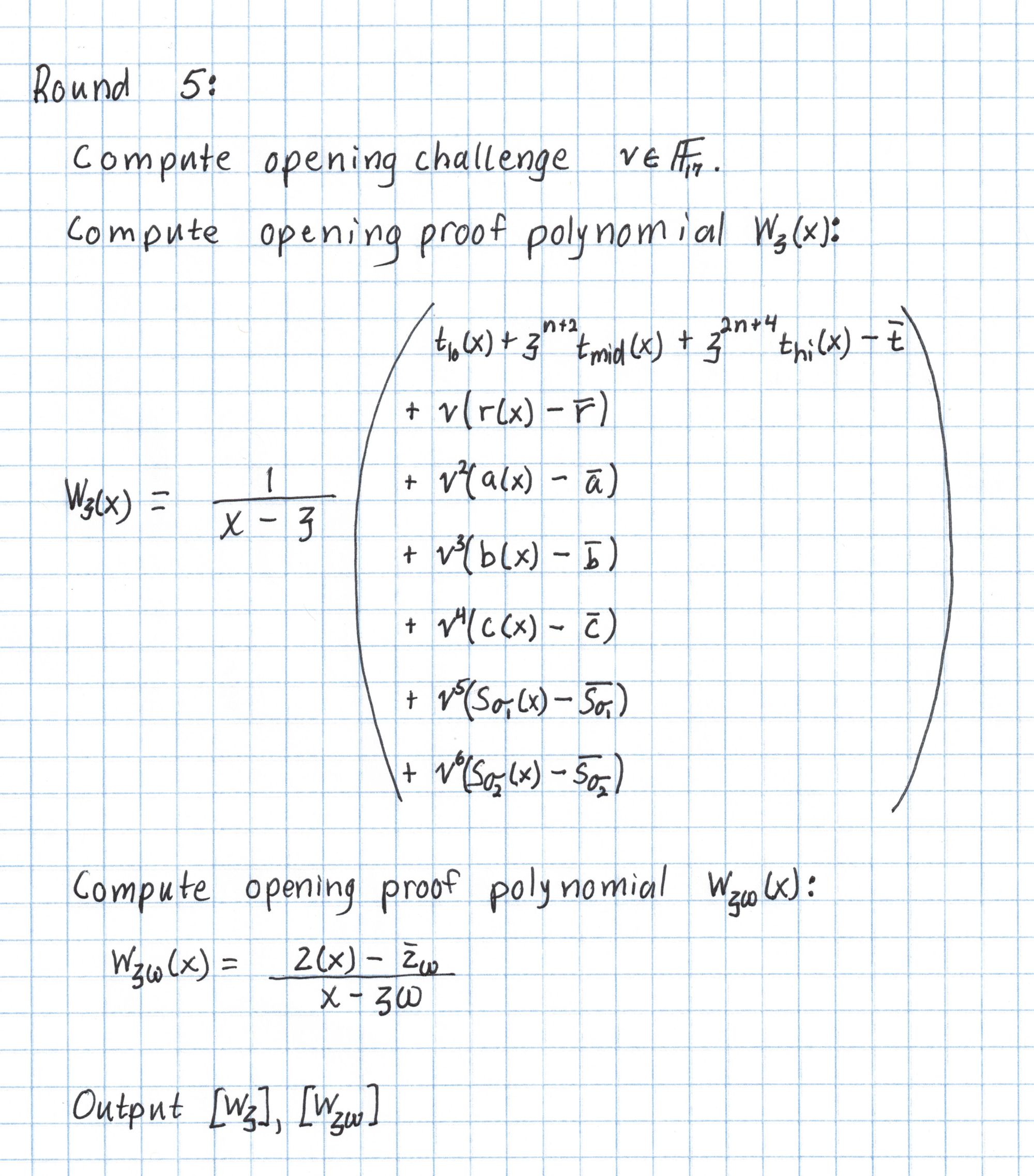
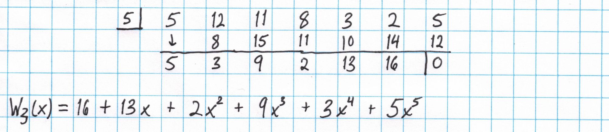
First we compute $W_\mathfrak{z}$. If you look carefully at the big sum on the right side, there are seven rows of polynomials each multiplied by a power of $v$. Each of these rows should have $\mathfrak{z}$ as a root. That means we should be able to evenly divide the whole sum by $x-\mathfrak{z}$ with no remainder.
We will compute the big sum first, then use synthetic division to divide by $x-\mathfrak{z}$. The polynomials are aligned so that the sum of each column gives the result on the final line.
Then we divide by $x-\mathfrak{z}$ using synthetic division.
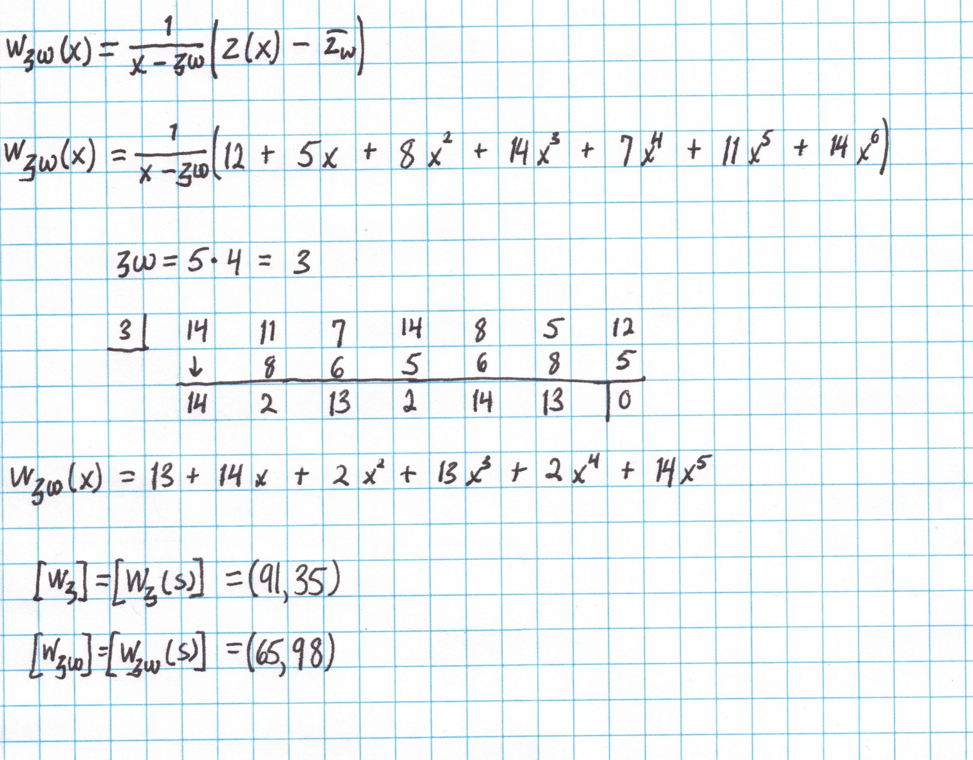
Now we compute the second polynomial $W_{\mathfrak{z}\omega}$, which will also require synthetic division. We evaluate each polynomial at the secret value $s$ using the SRS and output the two results.
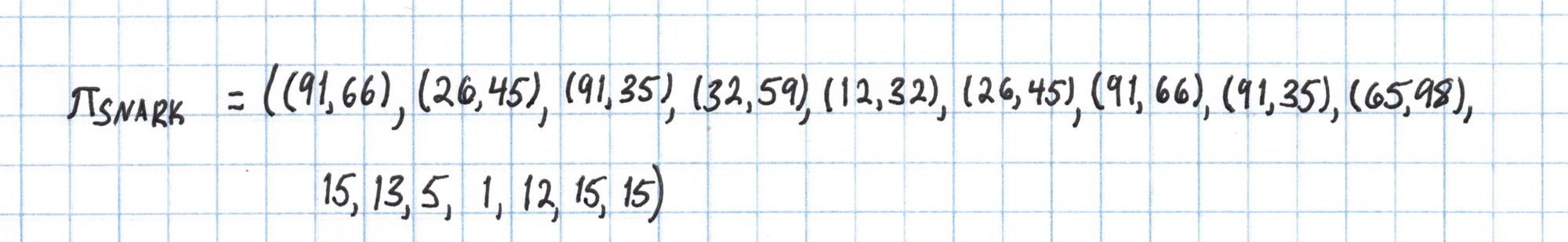
The Proof
We have now computed every element we need for the proof, called $\pi_{SNARK}$ below:
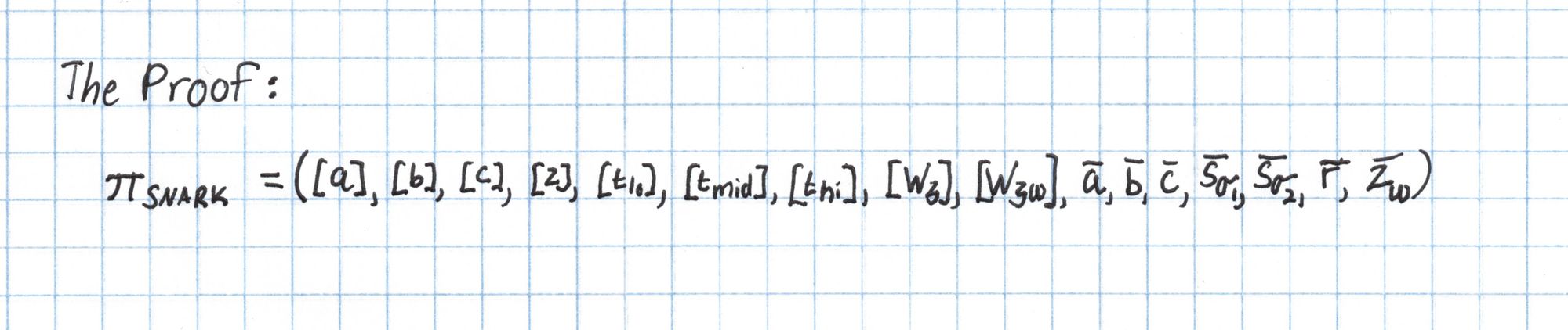
We'll use the the values for each of these components we computed earlier and send them to the Verifier as the completed proof.
Finally we have a proof! In the next section we will verify the proof using an elliptic curve pairing.
Written by Joshua Fitzgerald, zero-knowledge cryptography researcher & protocol developer at Metastate.
Image credits: Koala from Wikimedia.
Metastate has ceased its activities on the 31st of January 2021. The team members have joined a new company and working on a new project. If you're interested in zero-knowledge cryptography and cutting-edge cryptographic protocols engineering positions in Rust, check out the open positions at Heliax.
If you have any feedback or questions on this article, please do not hesitate to contact us: hello@heliax.dev.